Posts for January 2013

3D model: Inline-four engine

Thing practiced: 3D modeling

Tool used: SolidWorks 2013 trial

I’ve always had an iffy understanding of how car engines work – I learned pretty much everything I know (about everything) from this book when I was small. To understand better, I started modeling one in Solidworks:

Intake and exhaust camshafts:
Camshafts

Pistons and connecting rods:
Pistons and rods

Crankshaft:
Crankshaft

Classic AI: Mancala

Thing practiced: logic computers

Tools used: Sublime Text 3 beta, SWI-Prolog, J.R. Fisher’s Prolog tutorial

Mancala is a traditional African two-player board game with many different variations. One variant of mancala, called Kalah, has a long history in AI research – see e.g. Silver 1961 (pdf), Bell 1968, Slagle and Dixon 1969 (pdf), and Irving et al 2000 (pdf).

Prolog is a logic programming language devised by Alain Colmerauer and his colleagues in the early 1970s. The idea behind the language is that you feed the computer a set of facts and rules, then ask the computer to use those constraints to answer questions about things you want to know.

For today’s practice, I tried to implement a program to play mancala in Prolog – specifically the version of mancala I learned in elementary school day care, which has three seeds per hole (game rules are here). To solve the game, we can generate a tree of possible moves for each state and use minimax with alpha-beta pruning to find the optimal one. The code is here.

Data: Super Bowl pool squares

Tools used: RStudio with ggplot2, plyr, reshape2, and XML packages

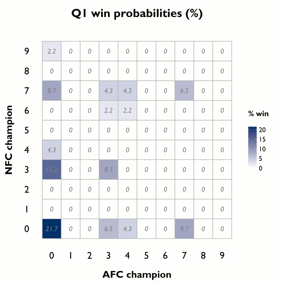
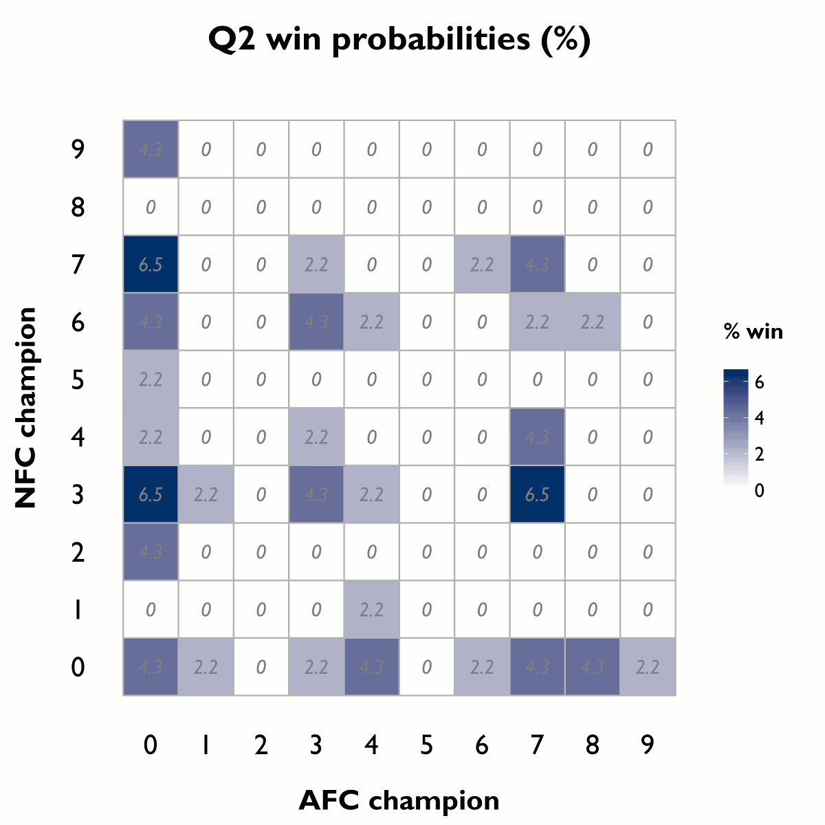
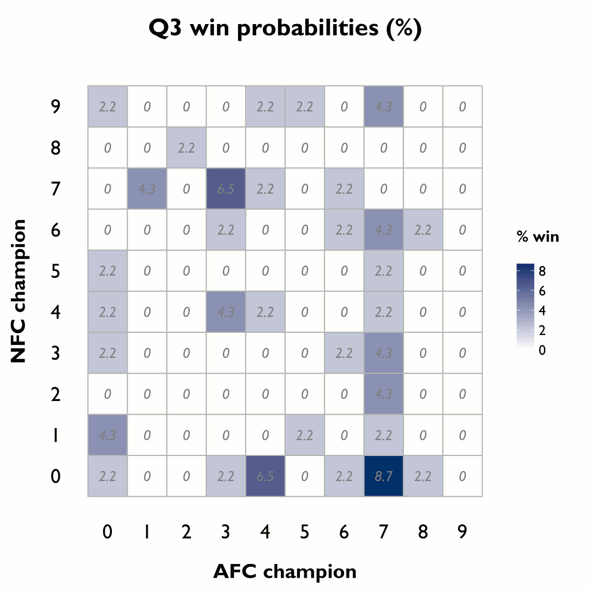
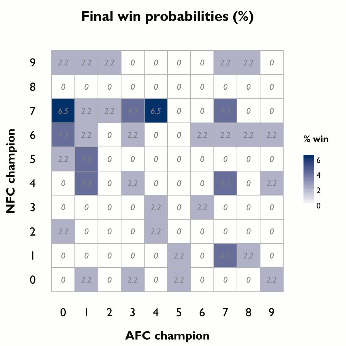
The way Super Bowl pools work, I’m told: people who buy in are randomly assigned a pair of numbers on a 10-by-10 grid. At the end of each quarter, the person with the box corresponding to the last digits of the two teams’ scores wins part of the pool.

Since some of us’ll be participating in a pool like this on Sunday, it might be useful to look at which numbers are most likely to be profitable.

Q1 Q2

.

Q3 Final

(R code here).

Photos: California coast

Thing practiced: photography

Tools used: Canon Digital Rebel T3i, Canon 40mm pancake lens, and a hat to keep my hair from flying into the shot

Point Reyes National Seashore Point Reyes National Seashore – f/2.8, 1/400 s, ISO 100

Julia Pfeiffer Burns State ParkPoint Reyes National Seashore
Julia Pfeiffer Burns State Park – f/8, 1/20 s, ISO 100
Point Reyes National Seashore – f/2.8, 1/2000 s, ISO 100

Limekiln State Park Limekiln State Park – f/2.8, 1/20 s, ISO 100

Web game: Pillow Fight!

Thing practiced: computers

Tools used: Sublime Text 2, Inkscape, Google Chrome

screenshotscreenshot

I was never much of a gamer, probably because I really suck at video games. I do remember spending an entire afternoon as a kid playing a Flash game about pancakes, though. For today’s practice I tried to replicate the pancake game, but in HTML5/JavaScript instead of Flash. And with pillows.

Try it here.

The goal: to earn points by arranging pillows into piles of the same color. You earn 100 points whenever you make a pile of three same-colored pillows. You can only move the topmost pillow in each stack. To move a pillow, touch the stack it’s in, then touch the stack you’d like to move it to. New pillows are added at an increasing rate as the game level increases, and the game ends when any stack reaches the top of the screen.

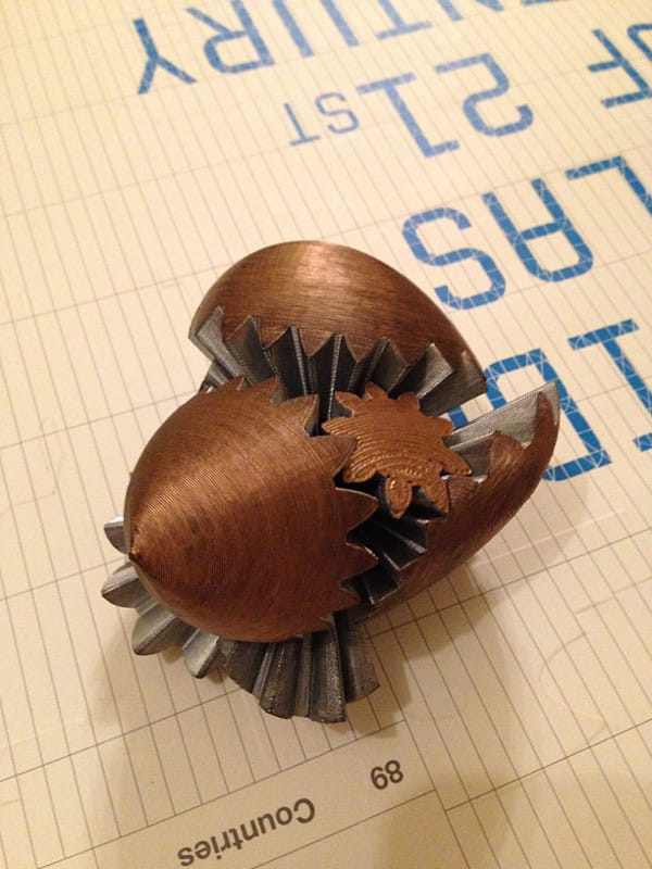
Thing: Heart gears

Thing practiced: nothing

Tools used: OpenSCAD, MakerBot Replicator

Modified and printed Emmett Lalish’s heart gears.

screwless heart gearsheartless screw gears

Photos: Around LA

Thing practiced: photography

Tools used: Canon Digital Rebel T3i with a Canon 40mm EF f/2.8 pancake lens and a Tiffen circular polarizer

Huntington Library - outside Huntington Library, near main gallery – f/2.8, 1/80 s, ISO 100 Huntington Library - rose garden Huntington Library, rose garden – f/2.8, 1/500 s, ISO 100 Huntington Library - Japanese garden Huntington Library, Japanese garden – f/2.8, 1/80 s, ISO 200 Huntington Library - Japanese garden Huntington Library, Japanese garden – f/2.8, 1/60 s, ISO 320

Huntington Library - bamboo forestHuntington Library - desert garden
Huntington Library, bamboo forest – f/2.8, 1/80 s, ISO 1600
Huntington Library, desert garden – f/2.8, 1/60 s, ISO 200

Huntington Library - lily pond Huntington Library, lily pond – f/2.8, 1/60 s, ISO 1600 Griffith Observatory Griffith Park, walk up to the observatory – f/2.8, 1/25 s, ISO 3200 Griffith Observatory Griffith Observatory, southeast view – f/2.8, 0.3 s, ISO 3200 Griffith Observatory Griffith Observatory, southeast view – f/2.8, 1/25 s, ISO 3200

Scientific computing: Fast Fourier transform

Thing practiced: computers

Tools used: Visual Studio 2012 on a Windows machine

(Quick background: The Fourier transform lets us translate any irregular signal into a combination of pure sine waves. The numerical version of this is the discrete Fourier transform (DFT), which is ubiquitous today – it’s responsible for jpegs and mp3s, among other things – thanks to the efficient fast Fourier transform (FFT) family of algorithms.)

Let’s try to implement the FFT in F#. First, here’s the naive DFT algorithm (a direct translation to code of the definition): $$ X_k = \sum_{n=0}^{N-1} {x_n}e^{\frac{-2{\pi}i}{N} kn} \tag{DFT} $$

let slow_dft xs =
    let N = Array.length xs
    [| for k in 0 .. N - 1 ->
           let mutable x_k = Complex.Zero
           for n = 0 to N - 1 do
               let a = 2.0 * Math.PI / float N *
                       float k * float n
               x_k <- x_k + xs.[n] *
                      Complex((cos a), (sin a))
           x_k |]

This gives an exact answer, but with poor performance – this has O(N2) time complexity. To improve performance, we first reduce problem scope by assuming that the number of input terms is an integral power of 2, letting us use the radix-2 DIT divide-and-conquer algorithm. This splits the DFT into two DFTs – a DFT of the even-numbered and a DFT of the odd-numbered terms:

$$ X_k = \sum_{m=0}^{\frac{N}{2} -1} {x_{2m}}e^{\frac{-2{\pi}i}{N} k(2m)} + \sum_{m=0}^{\frac{N}{2} -1} {x_{2m+1}}e^{\frac{-2{\pi}i}{N} k(2m+1)} $$

which gets rearranged as: $$ X_k = \left\{ \begin{array} {r@{\quad}l} E_k + e^{\frac{-2{\pi}i}{N} k}{O_k} & \mbox{if} & k < N/2 \\ E_{k-N/2} - e^{\frac{-2{\pi}i}{N} (k-N/2)}{O_{k-N/2}} & \mbox{if} & k \ge N/2 \end{array} \right. $$

This article explains further. Code:

let radix2_fft xs =
    let bit_rev arr =
        let N = Array.length arr
        let mutable j = 0
        let swap (a : _[]) i j =
            let tmp = a.[j]
            a.[j] <- a.[i]
            a.[i] <- tmp
        let rec helper m j =
            let m = m / 2
            let j = j ^^^ m
            if j &&& m = 0 then helper m j else j
        for i = 0 to N - 2 do
            if i < j then swap arr i j
            j <- helper N j
    let radix2_helper (xs : Complex[]) N j m =
        let t = Math.PI * float m / float j
        let a = Complex((cos t), (sin t))
        let mutable i = m
        while i < N do
            let x_i = xs.[i]
            let t = a * xs.[i+j]
            xs.[i] <- x_i + t
            xs.[i+j] <- x_i - t
            i <- i + 2 * j
    let N = Array.length xs
    bit_rev xs
    let mutable j = 1
    while j < N do
        for m = 0 to j - 1 do
            radix2_helper xs N j m
        j <- 2 * j

This is fast – O(n log n) – but only handles signals with lengths of integral powers of 2. To use the radix-2 algorithm for a signal of arbitrary length, we need to increase length to the next smallest power of 2. We can’t zero-pad the signal itself, but if we express the transform as a convolution then pad the convolution we’ll get an exact answer. (My hour’s up, but if you’re interested the convolution algorithm is explained here.)

Data graphic: Unemployment in the US

Thing practiced: data visualization

Tools used: RStudio, ggplot2, and Inkscape

For today’s practice I tried to recreate the graphics in Nathan Yau’s unemployment map from 2009 using R and ggplot2.

Code for the solution is here.

The Bureau of Labor Statistics makes state-, region-, county-, and city-level unemployment data available in flat files via FTP here. I used mapping data from the R maps library to draw the regions, but the county names there don’t match the BLS county names exactly – I removed references to “County”, “Parish”, and “City” in the county names to solve some of the mismatch problems, but a few counties are still missing. Also, I didn’t bother plotting and insetting Alaska or Hawaii.

The result (this would’ve been more interesting if I’d waited until the 2012 data was released, but still): unemployment choropleth

Project Euler: #108, Diophantine reciprocals

Thing practiced: math

Tools used: pen, paper, and MonoDevelop

Problem:

In the equation
$$ \frac{1}{x} + \frac{1}{y} = \frac{1}{n} \tag{1} $$ where x, y, and n are positive integers, what is the least value of n where the number of distinct solutions (i.e. solutions where x, y does not recur as y, x) exceeds 1000?

Solution:

Since x, y, and n are positive integers, we know that x and y must each be greater than n. Thus, we can rewrite (1) as
$$ \frac{1}{n+a} + \frac{1}{n+b} = \frac{1}{n} \tag{2} $$ where a and b are again positive integers.

Doing some algebra, we get:
$$ \frac{n+b}{(n+a)(n+b)} + \frac{n+a}{(n+a)(n+b)} = \frac{1}{n} \tag{3} $$ $$ n(2n+a+b) = (n+a)(n+b) \tag{4} $$ $$ n^2 = ab \tag{5} $$

This means that each distinct pair of divisors of n2 represents a distinct solution to (1). Thus, if we can find the number of divisors that n2 has, we’ll know that half that number (well, actually divisors(n2) + 1 / 2 because one of the divisor pairs – n * n = n2 – won’t be doubled) is the number of solutions to (1).

Now we just need an algorithm to find the number of divisors of a given integer m. An easy way to do this would be to enumerate each of the numbers up to sqrt(m) and count each number that divides m evenly as a divisor. Since we’re going to use this algorithm many times, though, this brute force approach won’t work.

Instead, we’ll use the divisor function. This tells us that we can obtain the number of divisors of m from its prime factorization. Specifically, the number of divisors of m is the product over all distinct prime factors of the power of the prime factor, plus 1. (That is, if we can write
$$ m = \prod^r_{i=1} p_i^{s_i} \tag{6} $$ then we have $$ d(m) = \prod^r_{i=1} (s_i + 1) \tag{7} $$ .) Think of it this way: each distinct divisor of m is some distinct combination of m’s prime factors, and each prime factor can appear 0, 1, …, or si times, so multiplying through for each of the prime factors we get (7).)

Now we just need an algorithm to factor a number into primes. We can use a (pseudo-)sieve of Eratosthenes to generate a seed list of potential primes:

// This is not optimized, and not the real sieve
// -- see Melissa E. O'Neill, The Genuine Sieve
// of Eratosthenes -- because it doesn't matter
// here and my brain hurts.

// Returns a list of primes up to a given maximum.
let primes max =
    let rec sieve list =
        match list with
        | [] -> []
        | hd :: rest ->
            hd :: (sieve <| List.filter (fun x -> x % hd <> 0) rest)
    sieve [ 2 .. max ]

We use the list of primes to obtain the prime factorization:

// Returns the prime factorization of a number
// as a list of tuples of (prime, exponent). This
// only looks for prime factors up to a given
// maximum. Again this isn't optimized, because
// it doesn't matter for this size of problem.
// Definitely won't work for #110 though.
let primeFactors m max =
    let rec primeFactorsHelper (m, factorsSoFar) primesToTest =
        let singleFactorHelper m p factorsSoFar =
            let rec exponentHelper m p e =
                if m % p = 0 then exponentHelper (m/p) p (e+1)
                else (m, e)
            let (rem, exp) = exponentHelper m p 0
            rem, (p, exp) :: factorsSoFar
        match primesToTest with
        | [] -> factorsSoFar
        | hd :: rest when hd > m -> factorsSoFar
        | hd :: rest when m % hd = 0 ->
            primeFactorsHelper (singleFactorHelper m hd factorsSoFar) rest
        | hd :: rest -> primeFactorsHelper (m, factorsSoFar) rest
    primeFactorsHelper (m, []) (primes max)

Factoring n2 still takes some time, though, as n2 grows much more quickly than n. Luckily, we can factor n instead. From (6) we can see that $$ m^2 = (\prod^r_{i=1} p_i^{s_i})^2 = \prod^r_{i=1} p_i^{2{s_i}} \tag{8} $$ so with the same combinatorics that gave us (7) we have
$$ d(m^2) = \prod^r_{i=1}(2{s_i} + 1) \tag{9} $$

Now, finally, we can find the solution using (9):

// Returns the number of solutions for a given n.
// This still only uses prime factors up to a
// given maximum.
let solutions m maxPrime =
    primeFactors m maxPrime
    |> List.fold (fun acc (p, e) -> acc * ((2*e) + 1)) 1

And obtain the solution using an (empirically-determined-to-be) appropriate max prime seed:

// Returns the solution, finally, I think.
let problem108answer =
    { 1 .. System.Int32.MaxValue }
    |> Seq.find (fun n -> (((solutions n 17) + 1) / 2) > 1000)

This gives us a final answer of 180,180.

Meant to have a crack at #110 today also, but this problem took an embarassingly long time to solve.

Sketch: Paris girls

Thing practiced: drawing

Tools used: index card, pencil, eraser, and two pens

Paris